The gpusim R package
The open-source gpusim R package provides fast functions for the simulation of gaussian random fields using graphics processing units.
Based on NVIDIA's CUDA framework our packages makes use of the cufft and curand libraries. Both, the generation of unconditional simulations as well as the following conditioning step is implemented for benefit from current GPU's architecture.
However, the performance of the simulation strongly depends on the avaiable hardware, the best speedup factors are achieved for large grids. You can find some performance analysis in [1].
The gpusim R package is built according to the well known packages fields [2] and gstat [3] and enables converting simulation results to sp [4] objects.
We would be happy if you let us know about your experiences while testing the package.
Using gpusim requires the latest R version and a appropriate GPU. You will also need latest graphics drivers including NVIDIA's CUDA libraries.
For compiling from source, you need NVIDIA's CUDA SDK. A detailed (but short) installation instruction can be found in the package vignette.
The current version is 0.01. Downloads for different platforms can be found using the link below.
For compiling from sources on Windows, you need a Microsoft Visual Studio 2010 Compiler, NVIDIA's CUDA Toolkit and NVIDIA's GPU Computing SDK.
Download Site
As a starting point for working with gpusim, have a look at the following R script, which generates 5 realizations of an unconditional simulation using an exponential covariance function.
Before you run the following script, make sure you have successfully installed gpusim by executing R CMD INSTALL gpusim in your Linux terminal or installing the package binaries using the Rgui in Windows.
library(gpusim) # <-- load R package
gpuDeviceInfo() # <-- print GPU capabilities
# define grid
xmin = 0
xmax = 5
ymin = 0
ymax = 5
nx = 100
ny = 100
dx = (xmax-xmin)/nx
dy = (ymax-ymin)/ny
grid = GridTopology(c(xmin,ymin), c(dx,dy), c(nx,ny))
# define covariance function
model = "Exp"
range = 0.5
sill = 3
nugget = 0
k = 5 # number of realizations
simGPU = gpuSim(grid, model, sill, range, nugget, k) # <-- run simulation
image.plot(simGPU[,,5]) # <-- plot 5-th realization
 |
 |
 |
|
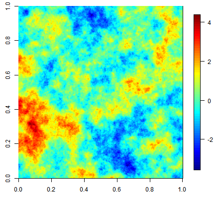
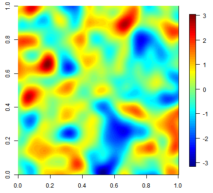
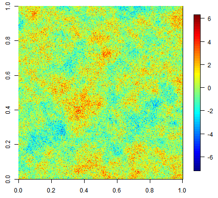
Three equiprobable realizations of an unconditional simulation on a 500x500 grid using an exponential covariance function.
|
 |
 |
 |
|
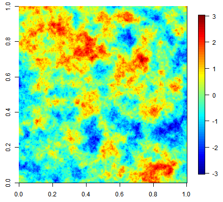
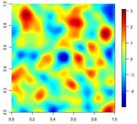
Three equiprobable realizations of an unconditional simulation on a 500x500 grid using a gaussian covariance function.
|
 |
 |
 |
|
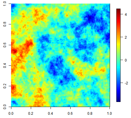
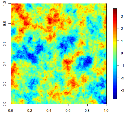
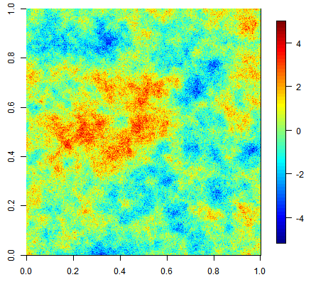
Three unconditional simulation results with the same exponential covariance function but increasing nugget effect
|
 |
 |
 |
|
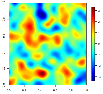
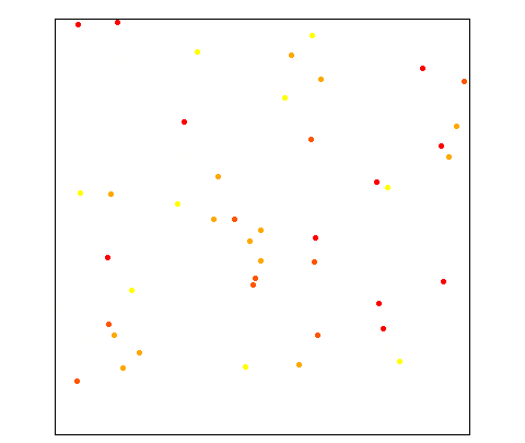
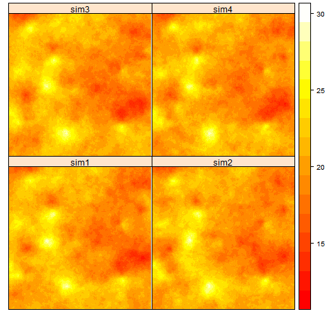
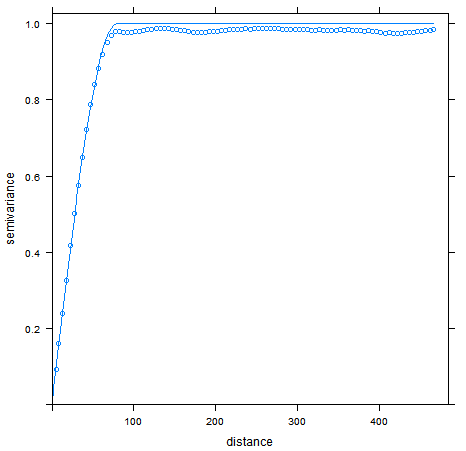
Conditional simulation on a 500x500 grid given 50 random points. The right figure compares the averaged resulting experimental variogram (points) of all realizations against the theoretical variogram model.
|
Katharina Henneboehl - katharina.henneboehl@uni-muenster.de
Marius Appel - marius.appel@uni-muenster.de
[1] -
[2] Reinhard Furrer, Douglas Nychka and Stephen Sain (2011). fields:
Tools for spatial data. R package version 6.6.1.
http://CRAN.R-project.org/package=fields
[3] Pebesma, E.J., 2004. Multivariable geostatistics in S: the gstat
package. Computers & Geosciences, 30: 683-691.
[4] Pebesma, E.J., R.S. Bivand, 2005. Classes and methods for spatial
data in R. R News 5 (2), http://cran.r-project.org/doc/Rnews/.